Dataset Description
The Committee on Earth Observation Satellites (CEOS) Atmospheric Composition – Virtual Constellation (AC-VC) GHG team has generated national top-down CO
2 budgets. This dataset is described by Byrne et al. (2022) and consists of:
- Top-down annual net land-atmosphere CO2 fluxes (NCE) from an ensemble of atmospheric CO2 inversions.
- Bottom-up estimates of fossil fuel emissions and lateral carbon fluxes due to crop trade, wood trade, and river export.
- Annual changes (loss) in terrestrial carbon stocks (ΔCloss) obtained by combining top-down and bottom-up estimates
In addition, two metrics are provided to help users interpret country-level data:
- The Z-statistics, which characterizes the differences between top-down NCE estimates.
- The Fractional Uncertainty Reduction (FUR), which characterizes the impact of assimilated CO2 data on reducing NCE uncertainties.
These data are provided for the period 2015-2020 on both a global grid and as country-level totals with error characterization. Figures 1 and 2 illustrates how these carbon fluxes relate to each other and the methodology is described in more detail below.
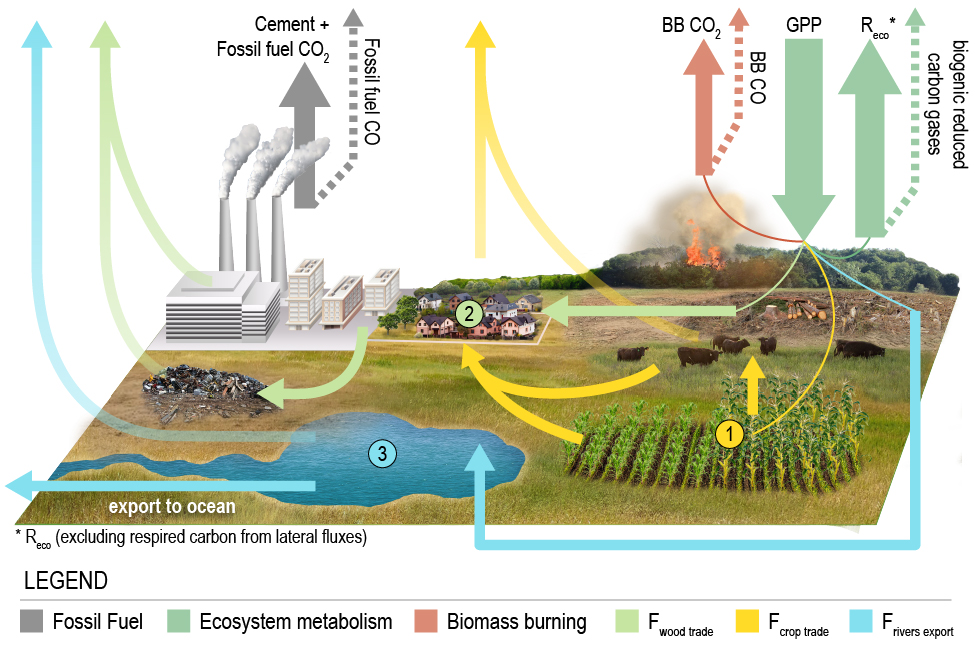 Figure 1. CO2 is removed from the atmosphere through photosynthesis (GPP) and then emitted back to the atmosphere through a number of processes. Three processes move carbon laterally on Earth’s surface, such that emissions of CO2 occur in a different region than removals: (1) Agriculture; harvested crops are transported to urban areas and to livestock, which are themselves exported to urban areas. CO2 is respired to the atmosphere in livestock or urban areas. (2) Forestry; logged carbon is transported to urban and industrial areas, then emitted to through decomposition in a landfill or combustion as a biofuel. (3) Water cycle; carbon is leached from soils into water bodies, such as lakes. The carbon is then either deposited, released to the atmosphere, or transported to the ocean. Arrows show carbon fluxes and colors indicate whether the flux is associated with (grey) fossil fuel emissions, (dark green) ecosystem metabolism, (red) biomass burning, (light green) forestry, (yellow) agriculture, or (blue) the water cycle. Semi-transparent arrows show fluxes that move between the surface and atmosphere, while solid arrows show fluxes that move between land regions. Dashed arrows show surface-atmosphere fluxes of reduced carbon species that are oxidized to CO2 in the atmosphere. For simplicity, a cement carbonation sink, volcano emissions, and a weathering sink are not included in this figure.
Methodology
Top-down NCE estimates are obtained from an ensemble of state-of-the-art flux inversion systems participating in the OCO-2 v10 Model Intercomparison Project (
v10 OCO-2 MIP). The atmospheric CO
2 inversion systems provide spatially- and temporally-resolved estimates of surface-atmosphere fluxes for land and oceans from which country level annual land-atmosphere CO
2 fluxes can be estimated. Flux estimates are provided for four experiments that differ in the atmospheric CO
2 datasets used to constrain fluxes. These experiments estimate surface-atmosphere CO
2 fluxes using:
- IS: in situ CO2 measurements in the National Oceanic and Atmospheric Administration (NOAA) Observation Package (ObsPack; https://gml.noaa.gov/ccgg/obspack/).
- LNLG: column-averaged CO2 dry air mole fraction, XCO2, retrievals over land NASA Orbiting Carbon Observatory-2 (OCO-2).
- LNLGIS: both in situ CO2 and OCO-2 land XCO2 data.
- LNLGOGIS: in situ CO2, OCO-2 land XCO2, and OCO-2 ocean XCO2 data combined.
For each experiment, NCE and ocean CO
2 fluxes are optimized to match the atmospheric CO
2 observations within their uncertainties. The net biosphere exchange (NBE) is calculated by subtracting bottom-up fossil fuel emission estimates from NCE, as the inversions cannot clearly discriminate emissions from fossil fuel and biosphere-atmosphere fluxes, and the fossil fuel CO
2 sources are generally much better known. Thus, bottom-up fossil fuel emission estimates are subtracted from NCE estimate to obtain biosphere-atmosphere fluxes. The net loss of land carbon is then estimated by accounting for “lateral” carbon fluxes from the terrestrial biosphere such as land-to-ocean transport of carbon by rivers (a natural process perturbed by human activities) and the import and export of harvested agricultural and wood products (a human activity). Changes in terrestrial carbon stocks (ΔC
loss) reflect the combined impact of direct anthropogenic activities and changes to managed ecosystems in response to rising atmospheric CO
2 concentrations, climate change, and disturbances (i.e., droughts, floods, wildfires, severe weather). Figure 2 shows how each of these CO
2 fluxes relate to each other and desired quantities.
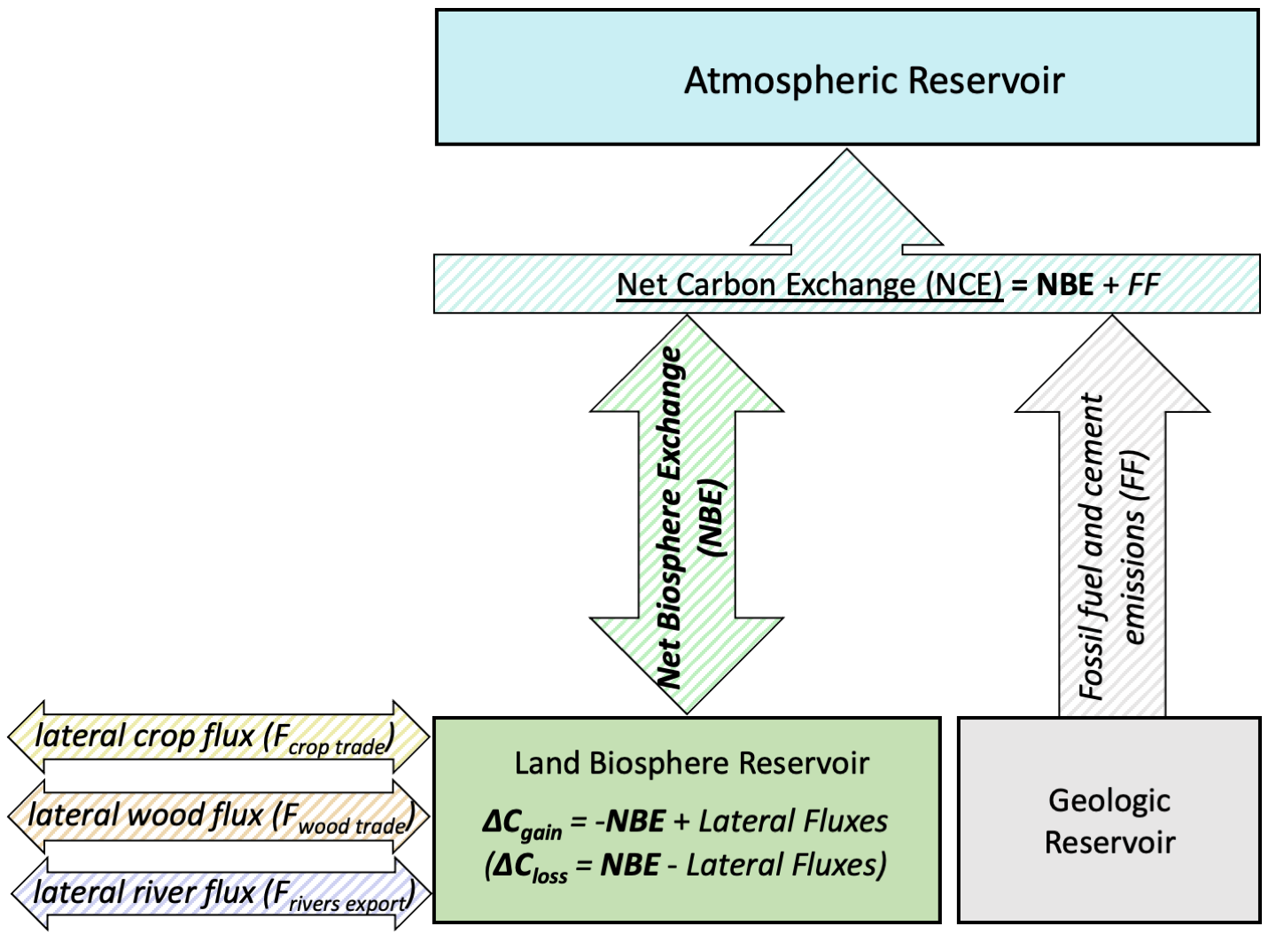 Figure 2. Carbon fluxes for a given land region, such as a country. Boxes with solid backgrounds show reservoirs of carbon. Arrows with hatched shading show fluxes between reservoirs. NCE is underlined to emphasize that this quantity is estimated from the atmospheric CO2 measurements using top-down methods. Italicized quantities are obtained from bottom-up datasets (FF, Fcrop trade, Fwood trade, Frivers export). Bold quantities are derived in this study from the top-down and bottom-up datasets (NBE, ΔCgain, ΔCloss).
Summary of Results
This dataset provides global gridded and country-level totals of NCE, and ΔC
loss from four OCO-2 MIP experiments, as well as bottom-up fossil fuel emissions and lateral flux estimates over 2015-2020. Here we present a sample of the fluxes provided in this dataset. Figure 3 shows the 2015-2020 gridded and country-scale NCE and ΔC
loss for the LNLGIS experiment. At 1x1 degree (Fig 3a-b), localized fossil fuel emissions are visible, generally corresponding to urban areas and industrialized regions. These emissions are interspersed over broad source and sink structures that are driven by biosphere uptake or release. Land biosphere uptake is most evident across the northern mid-high latitudes. In contrast, tropical uptake and release is more regional. Aggregating NCE to country-scale (Fig. 3c-d), most countries are net sources driven by fossil fuel emissions, particularly in the northern extratropics. Figure 3e-f shows the 2015-2020 mean country-level ΔC
loss for the LNLGIS experiment. Carbon uptake by land is found for most extratropical countries, while tropical countries can either be sources or sinks. Notably, the uncertainty in ΔC
loss is larger in the tropics, particularly for mid-sized countries. Overall, small to mid-sized countries generally have uncertainties comparable to the magnitude of ΔC
loss, reflecting the fact that atmospheric CO
2 measurements best constrain fluxes over large scales.
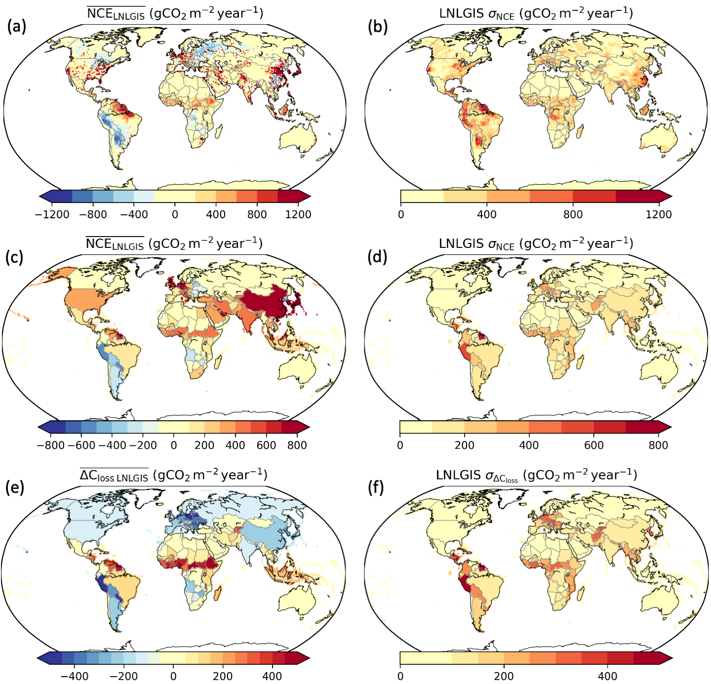 Figure 3. Median and standard deviation of NCE on a (a-b) 1x1 degree grid and (c-d) aggregated to country-scale for the v10 OCO-2 MIP LNLGIS experiment over 2015-2020. (e-f) Median and standard deviation of country-scale ΔCloss over 2015-2020 derived from the LNLGIS OCO-2 v10 MIP experiment.
Figure 4 shows carbon budgets over 2015-2020 for four countries (USA, India, Indonesia, and Australia). All of the CO
2 fluxes on the left of the dashed line (FF, lateral fluxes, ΔC
loss) combine to give the NCE flux constrained by the OCO-2 MIP experiments. We find that FF is the strongest contributor to NCE for all countries, but that ΔC
loss also plays a strong modulating role. For example, negative ΔC
loss for the USA (carbon uptake by the land biosphere) reduces NCE to be less than would be expected given the FF emissions. Conversely, Indonesia has positive ΔC
loss (loss of carbon from land biosphere), resulting in increased NCE relative to FF. Some countries also show differences in ΔC
loss between OCO-2 MIP experiments. For example, the LNLG and LNLGIS experiments suggest negative ΔC
loss for India, while the IS suggest ΔC
loss is roughly neutral.
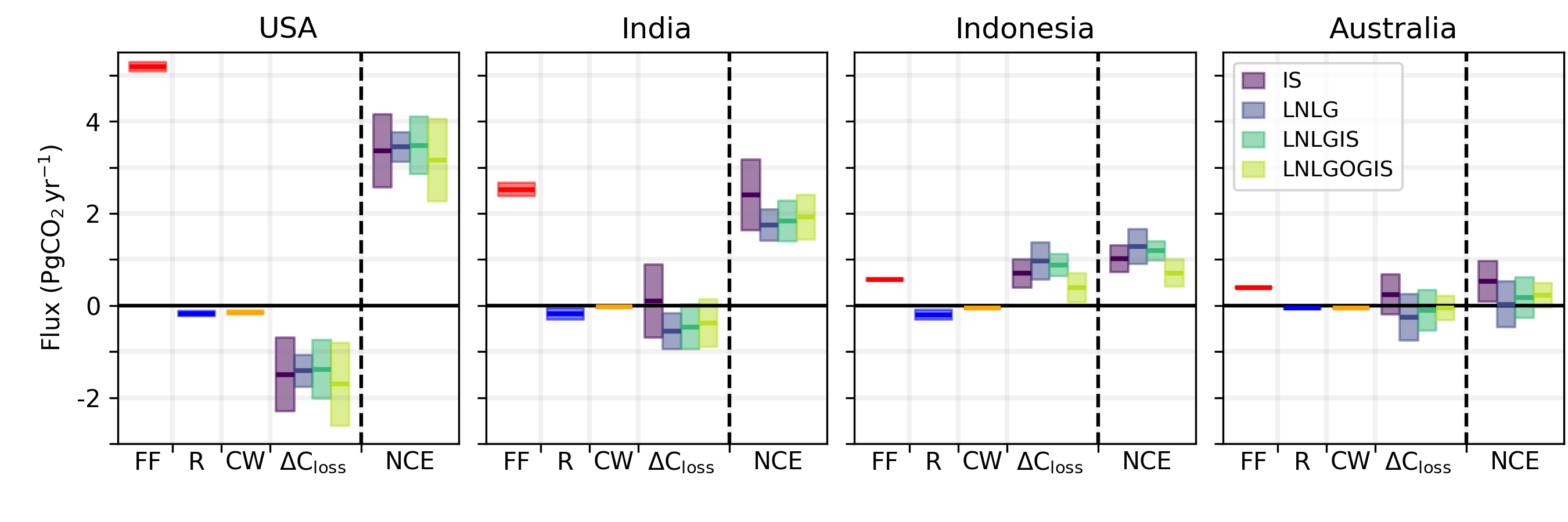 Figure 4. 2015-2020 carbon budget for the USA, India, Indonesia, and Australia. Bars show the median +/- standard deviation of FF, Frivers export (R), Fcrop trade + Fwood trade (CW), ΔCloss, and NCE.
The carbon budgets can also be examined for individual years (Fig. 5). Both Indonesia and Australia show considerable variations in ΔC
loss that drive variations in NCE over this period. Indonesia has a large positive ΔC
loss in 2015 driven by warm-dry weather and fires during 2015 El Niño. Australia showed strong negative ΔC
loss (except for IS) during 2016, which was the 15th wettest year on record but positive ΔC
loss during 2019, which was the warmest and driest year on record. Variations in NCE are also driven by variations in FF emissions. In particular, a reduction in NCE is found for 2019 and 2020 in the USA that is primarily linked to a reduction in FF emissions rather than ΔC
loss.
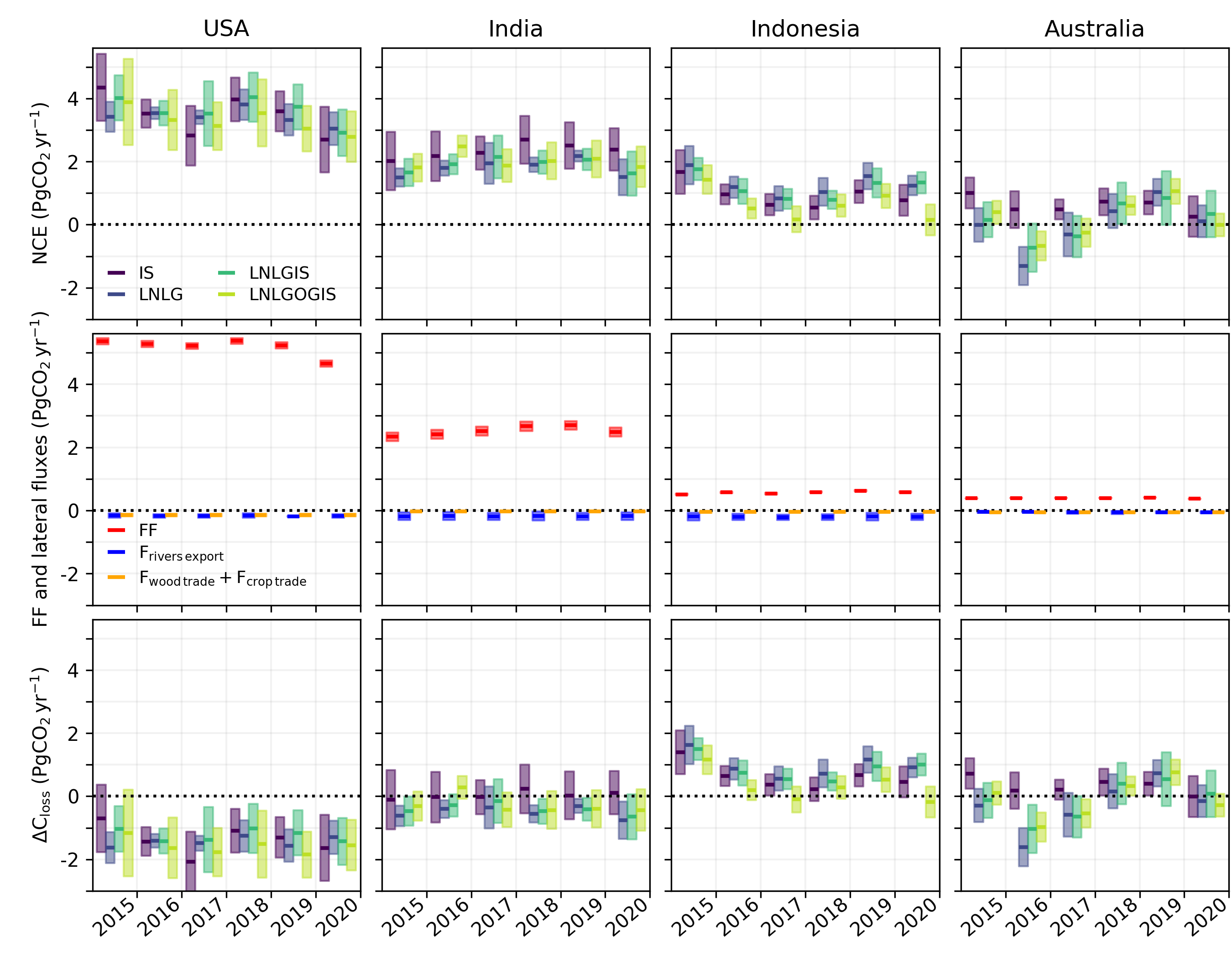 Figure 5. Timeseries of the carbon budget for the USA, India, Indonesia, and Australia. Solid lines show the median estimates and shaded areas show +/- 1 standard deviation.
For future stocktakes, these estimates will be refined as new space-based observing systems are deployed. Future atmospheric CO
2 observing systems are expected to dramatically improve the resolution and coverage, facilitating inversions that could simultaneously constrain fossil fuel and AFOLU emissions. Complimentary expansions of ground-based and aircraft-based CO
2 measurements are critically needed in under-sampled regions both to complement the coverage of the space-based data and to assess their accuracy. Improvements to flux inversion systems will also further refine results, as reductions to systematic transport errors will be critical for refining carbon flux estimates.
Citation: Byrne, B., Baker, D. F., Basu, S., Bertolacci, M., Bowman, K. W., Carroll, D., Chatterjee, A., Chevallier, F., Ciais, P., Cressie, N., Crisp, D., Crowell, S., Deng, F., Deng, Z., Deutscher, N. M., Dubey, M. K., Feng, S., García, O. E., Herkommer, B., Hu, L., Jacobson, A. R., Janardanan, R., Jeong, S., Johnson, M. S., Jones, D. B. A., Kivi, R., Liu, J., Liu, Z., Maksyutov, S., Miller, J. B., Miller, S. M., Morino, I., Notholt, J., Oda, T., O’Dell, C. W., Oh, Y.-S., Ohyama, H., Patra, P. K., Peiro, H., Petri, C., Philip, S., Pollard, D. F., Poulter, B., Remaud, M., Schuh, A., Sha, M. K., Shiomi, K., Strong, K., Sweeney, C., Té, Y., Tian, H., Velazco, V. A., Vrekoussis, M., Warneke, T., Worden, J. R., Wunch, D., Yao, Y., Yun, J., Zammit-Mangion, A., and Zeng, N.: Pilot top-down CO2 Budget constrained by the v10 OCO-2 MIP Version 1, Committee on Earth Observing Satellites, https://doi.org/10.48588/npf6-sw92, Version 1.0, 2022